Transform data with Flux
This page documents an earlier version of InfluxDB. InfluxDB v2.1 is the latest stable version. See the equivalent InfluxDB v2.1 documentation: Transform data with Flux.
When querying data from InfluxDB, you often need to transform that data in some way. Common examples are aggregating data into averages, downsampling data, etc.
This guide demonstrates using Flux functions to transform your data.
It walks through creating a Flux script that partitions data into windows of time,
averages the _values in each window, and outputs the averages as a new table.
It’s important to understand how the “shape” of your data changes through each of these operations.
Query data
Use the query built in the previous Query data from InfluxDB guide, but update the range to pull data from the last hour:
from(bucket:"telegraf/autogen")
  |> range(start: -1h)
  |> filter(fn: (r) =>
    r._measurement == "cpu" and
    r._field == "usage_system" and
    r.cpu == "cpu-total"
  )
Flux functions
Flux provides a number of functions that perform specific operations, transformations, and tasks. You can also create custom functions in your Flux queries. Functions are covered in detail in the Flux functions documentation.
A common type of function used when transforming data queried from InfluxDB is an aggregate function.
Aggregate functions take a set of _values in a table, aggregate them, and transform
them into a new value.
This example uses the mean() function
to average values within time windows.
The following example walks through the steps required to window and aggregate data, but there is a
aggregateWindow()helper function that does it for you. It’s just good to understand the steps in the process.
Window your data
Flux’s window() function partitions records based on a time value.
Use the every parameter to define a duration of time for each window.
Calendar months and years
every supports all valid duration units,
including calendar months (1mo) and years (1y).
For this example, window data in five minute intervals (5m).
from(bucket:"telegraf/autogen")
  |> range(start: -1h)
  |> filter(fn: (r) =>
    r._measurement == "cpu" and
    r._field == "usage_system" and
    r.cpu == "cpu-total"
  )
  |> window(every: 5m)
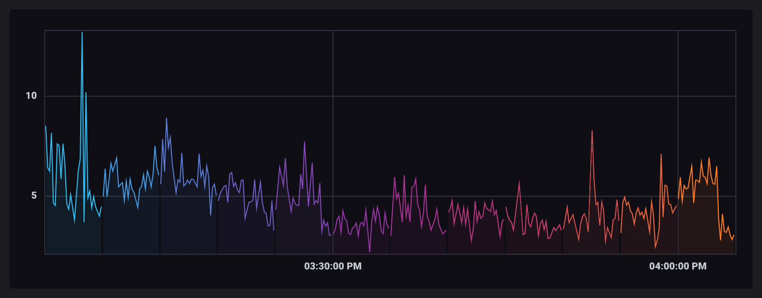
As data is gathered into windows of time, each window is output as its own table. When visualized, each table is assigned a unique color.

Aggregate windowed data
Flux aggregate functions take the _values in each table and aggregate them in some way.
Use the mean() function to average the _values of each table.
from(bucket:"telegraf/autogen")
  |> range(start: -1h)
  |> filter(fn: (r) =>
    r._measurement == "cpu" and
    r._field == "usage_system" and
    r.cpu == "cpu-total"
  )
  |> window(every: 5m)
  |> mean()
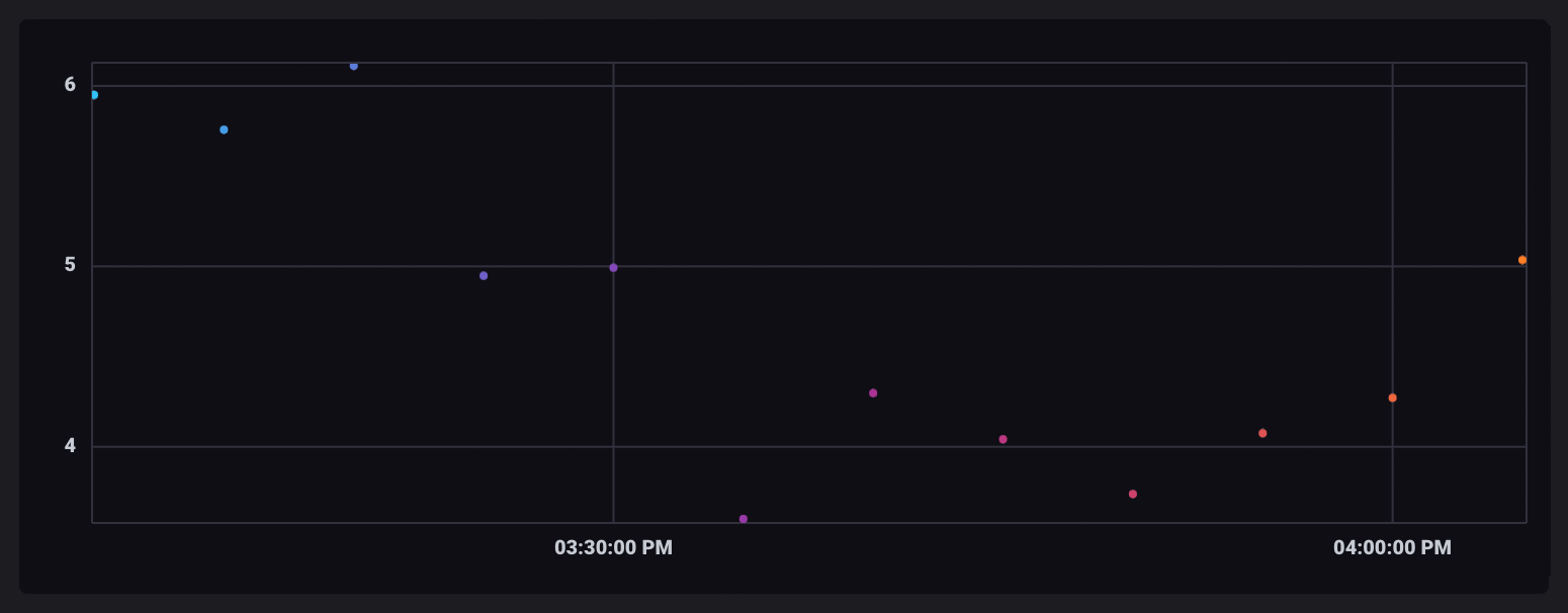
As rows in each window are aggregated, their output table contains only a single row with the aggregate value. Windowed tables are all still separate and, when visualized, will appear as single, unconnected points.

Add times to your aggregates
As values are aggregated, the resulting tables do not have a _time column because
the records used for the aggregation all have different timestamps.
Aggregate functions don’t infer what time should be used for the aggregate value.
Therefore the _time column is dropped.
A _time column is required in the next operation.
To add one, use the duplicate() function
to duplicate the _stop column as the _time column for each windowed table.
from(bucket:"telegraf/autogen")
  |> range(start: -1h)
  |> filter(fn: (r) =>
    r._measurement == "cpu" and
    r._field == "usage_system" and
    r.cpu == "cpu-total"
  )
  |> window(every: 5m)
  |> mean()
  |> duplicate(column: "_stop", as: "_time")
Unwindow aggregate tables
Use the window() function with the every: inf parameter to gather all points
into a single, infinite window.
from(bucket:"telegraf/autogen")
  |> range(start: -1h)
  |> filter(fn: (r) =>
    r._measurement == "cpu" and
    r._field == "usage_system" and
    r.cpu == "cpu-total"
  )
  |> window(every: 5m)
  |> mean()
  |> duplicate(column: "_stop", as: "_time")
  |> window(every: inf)
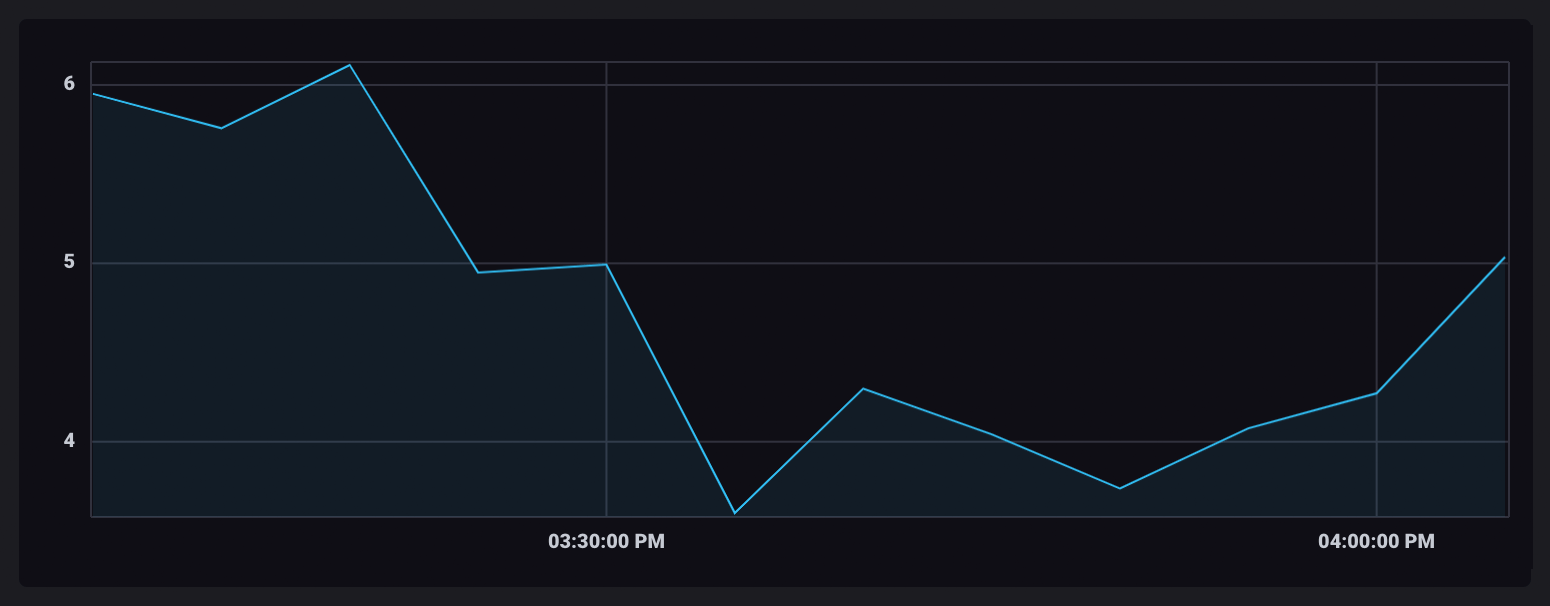
Once ungrouped and combined into a single table, the aggregate data points will appear connected in your visualization.

Helper functions
This may seem like a lot of coding just to build a query that aggregates data, however going through the process helps to understand how data changes “shape” as it is passed through each function.
Flux provides (and allows you to create) “helper” functions that abstract many of these steps.
The same operation performed in this guide can be accomplished using the
aggregateWindow() function.
from(bucket:"telegraf/autogen")
  |> range(start: -1h)
  |> filter(fn: (r) =>
    r._measurement == "cpu" and
    r._field == "usage_system" and
    r.cpu == "cpu-total"
  )
  |> aggregateWindow(every: 5m, fn: mean)
Congratulations!
You have now constructed a Flux query that uses Flux functions to transform your data. There are many more ways to manipulate your data using both Flux’s primitive functions and your own custom functions, but this is a good introduction into the basic syntax and query structure.
For a deeper dive into windowing and aggregating data with example data output for each transformation, view the Windowing and aggregating data guide.
Support and feedback
Thank you for being part of our community! We welcome and encourage your feedback and bug reports for InfluxDB and this documentation. To find support, the following resources are available:
InfluxDB Cloud and InfluxDB Enterprise customers can contact InfluxData Support.